Tutorial: PN junction¶

In this tutorial a simple model of PN junction will be constructed. The same model is used in example included in oedes distribution in file examples/interactive/pn.ipynb.

oedes contains models of typical devices. However, in this tutorial, the model will be constructed equation-by-equation to demonstrate basic functionality.

Importing oedes¶

Before starting, oedes package must be imported

>>> import oedes

The drift-diffusion system¶

For simulating transport, a model of temperature distribution must be assumed. In the simplest case of isothermal simulation, the same effective temperature is assumed equal everywhere inside the device. The model is created as follows:

>>> temperature = oedes.models.ConstTemperature()

The specification of model is separated from the specification of parameter values. The actual value of temperature, in Kelvins, will be given later.

The next step is to create Poisson’s equation of electrostatics

>>> poisson = oedes.models.PoissonEquation()

Constructed objects poisson and temperature must are passed as arguments when creating transport equations:

>>> electron = oedes.models.equations.BandTransport(poisson=poisson, name='electron', z=-1, thermal=temperature)
>>> hole = oedes.models.equations.BandTransport(poisson=poisson, name='hole', z=1, thermal=temperature)

Above creates two conventional drift-diffusion equations for electrons and holes respectively. By default, the mobility is assumed constant and the DOS is modeled by using the Boltzmann approximation. name arguments are names which are used to identify parameters and outputs. z are charges of species expressed in units of elementary charge. oedes allows arbitrary number of species, and arbitrary values of name and z. This allows to construct complicated models with, for example, mixed ionic-electronic transport.

The doping profile¶

To model the PN junction, a doping profile must be defined. In the example, left half of the device is doped with ionized donor concentration given by parameter Nd, and right half of device is doped with doped with ionized acceptor concentration given by parameter Na.

The pn_doping function is called during model evaluation and is given as parameters the mesh, the evaluation context object ctx, and the discretized equation object eq. In the example, it uses ctx object to access parameters values of the dopant concentations ('Na', ''Nd').

>>> def pn_doping(mesh, ctx, eq):
...     return oedes.ad.where(mesh.x<mesh.length*0.5,ctx.param(eq, 'Nd'),- ctx.param(eq, 'Na'))
>>> doping = oedes.models.FixedCharge(poisson, density=pn_doping)

The dopants are assumed to be fully ionized and therefore it is modeled as fixed charge. The FixedCharge adds calculated doping profile to the previously created Poisson’s equation poisson.

Above code uses a specialized version of function where is used instead of version from numpy. This is required for support of sensitivity analysis with respect to parameter values.

The Ohmic contacts¶

To keep the example simple, Ohmic contacts are assumed on both sides of the device. They are created as follows:

>>> semiconductor = oedes.models.Electroneutrality([electron, hole, doping],name='semiconductor')
>>> anode = oedes.models.OhmicContact(poisson, semiconductor, 'electrode0')
>>> cathode = oedes.models.OhmicContact(poisson, semiconductor, 'electrode1')

Ohmic contacts require knowledge of equilibrium charge carrier concentrations in semiconductor. This is calculated by Electroneutrality. Note that since concentrations in doped semiconductor are of interest, all charged species are passed to Electroneutrality. 'electrode0' and 'electrode1' refers to names of boundaries in the mesh.

Putting all together¶

To avoid divergence of the simulation due to infinitely large lifetime of electrons and holes, recombination should be added. Duirecrecombination model is created by

>>> recombination = oedes.models.DirectRecombination(semiconductor)

The calculation of terminal current is a non-trivial post-processing step. It is recommended to use Ramo-Shockley current calculation in most cases, which is created by

>>> current = oedes.models.RamoShockleyCurrentCalculation([poisson])

The discrete model is constructed and initialized by calling oedes.fvm.discretize. It takes two arguments: the system of equations and terms to solve, and the specification of domain. Below oedes.fvm.mesh1d creates a 1-D domain with length specified as argument.

>>> all_equations_and_terms = [ poisson, temperature, electron, hole, doping, current, semiconductor, anode, cathode, recombination ]
>>> domain = oedes.fvm.mesh1d(100e-9)
>>> model = oedes.fvm.discretize(all_equations_and_terms, domain)

Parameters¶

The physical parameters are provided as dict.

>>> params={
...     'T':300,
...     'epsilon_r':12,
...     'Na':1e24,
...     'Nd':1e24,
...     'hole.mu':1,
...     'electron.mu':1,
...     'hole.energy':-1.1,
...     'electron.energy':0,
...     'electrode0.voltage':0,
...     'electrode1.voltage':0,
...     'hole.N0':1e27,
...     'electron.N0':1e27,
...     'beta':1e-9
... }

Above, 'T' key is used to specify temperature in Kelvins. It is used by ConstTemperature object. 'epsilon_r' specifies the relative dielectric permittivity. It is used by discretized PoissonEquation object. 'Na' and 'Nd' are parameters accessed by pn_doping function, the concentrations of dopants. 'beta' is used by DirectRecombination.

Other parameters are in form name.parameter. name is passed to the equation, and they can be nested. For example, if a transport equation were created as

something = oedes.models.BandTransport(name='zzz',...)

then the corresponding mobility parameter would be identified by key 'zzz.mu'.

The mobilities electron.mu and hole.mu are given in $\mathrm{m^2 V^{-1} s^{-1}}$ , therefore are equal to 1000 $\mathrm{cm^2 V^{-1} s^{-1}}$ each. In the example above, instead of specifying electron affinity and band-gap, the energies of both bands are specified directly by energy parameters, in eV. The voltages are applied to Ohmic contacts are specified by 'electrode0.voltage' and 'electrode1.voltage', in Volts. N0 denotes the total density of states, in $\mathrm{m^{-3}}$ .

params¶

By convention, values of physical parameters are specified in dict object named params, with string keys, and float values. All values of given in SI base units, except for small energies which are specified in eV. oedes currently does not assume default values of parameters. If any necessary parameter is not specified in params, exception KeyError is raised.

Solving¶

oedes.context objects binds models with their parameters and solutions. It also provides convenience functions for solving, post-processing and plotting the data.

The following calculates soltuion for parameters specified in dict params

>>> c = oedes.context(model)
>>> c.solve(params)

Examining output¶

The solution can be investigated by calling output function, which returns a dict of available outputs:

>>> out=c.output()
>>> print(sorted(out.keys()))
['.meta', 'D', 'Dt', 'E', 'Et', 'J', 'R', 'c', 'charge', 'electrode0.J', 'electrode1.J', 'electron.Eband', 'electron.Ef', 'electron.J', 'electron.Jdiff', 'electron.Jdrift', 'electron.c', 'electron.charge', 'electron.ct', 'electron.j', 'electron.jdiff', 'electron.jdrift', 'electron.phi_band', 'electron.phi_f', 'hole.Eband', 'hole.Ef', 'hole.J', 'hole.Jdiff', 'hole.Jdrift', 'hole.c', 'hole.charge', 'hole.ct', 'hole.j', 'hole.jdiff', 'hole.jdrift', 'hole.phi_band', 'hole.phi_f', 'potential', 'semiconductor.Ef', 'semiconductor.electron.c', 'semiconductor.hole.c', 'semiconductor.phi', 'total_charge_density']

The outputs are numpy arrays. For example, the electrostatic potential is

>>> print(out['potential'])
[-0.17857923 -0.17858006 -0.17858115 -0.17858258 -0.17858445 -0.17858693
  -0.17859023 -0.17859468 -0.1785994  -0.17860442 -0.17860982 -0.17861567
  ...
  -0.92141696 -0.92141772]

To access additional information about output (such as its mesh), use .meta subdictionary.

>>> out['.meta']['potential']
OutputMeta(mesh=<oedes.fvm.mesh.mesh1d object at ...>, face=False, unit='V')

outputs¶

Most useful outputs are given below. Just as for params, all values are in SI base units, except for small energies in eV. * denotes prefix identifying the equation, such as electron or hole.

*.c: concentration of particles, in $\mathrm{m^{-3}}$
*.j: flux of particles, in $\mathrm{m^{-2} s^{-1}}$
*.Ef: quasi Fermi level, in eV
*.Eband: band energy, in eV
R: recombination density, in $\mathrm{m^{-3} s^{-1}}$
J: total electric current density, in $\mathrm{A m^{-2}}$
E: electric field, in V/m
potential: electrostatic potential, V

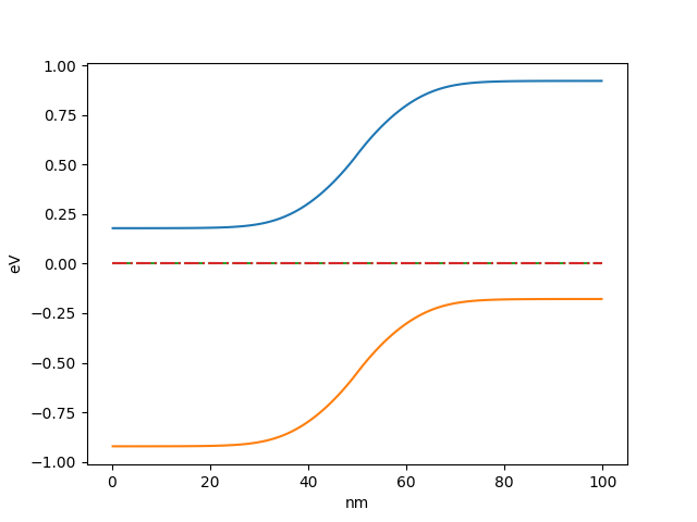
Plotting¶

oedes.context object simplifies plotting results using matplotlib. For example, bands and quasi Fermi levels are plotted as

>>> import matplotlib.pylab as plt
>>> fig,ax = plt.subplots()
>>> p=c.mpl(fig, ax)
>>> p.plot(['electron.Eband'],label='$E_c$')
>>> p.plot(['hole.Eband'],label='$E_v$')
>>> p.plot(['electron.Ef'],linestyle='--',label='$E_{Fn}$')
>>> p.plot(['hole.Ef'],linestyle='-.',label='$E_{Fp}$')
>>> p.apply_settings({'xunit':'n','xlabel':'nm'})