Physical models¶

Concentrations of charges in thermal equilibrium¶

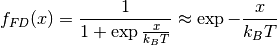
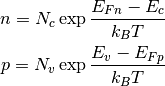
Probability $f_{FD}$ that an electronic state with energy $E$ is occupied is given by the Fermi-Dirac distribution:

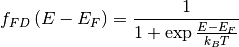
$f_{FD} \left ( E - E_F \right) = \frac{1} {1+\exp \frac{E-E_F}{k_B T}}$

with $E_F$ denoting the Fermi energy, $k_B$ denoting the Boltzmann constant and $T$ denoting the temperature.

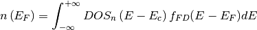
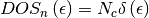
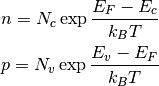
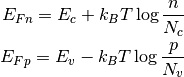
The states in the conduction band are distributed in energy according to the density of states function 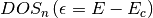$DOS_n \left( \epsilon = E - E_c \right)$ . The total concentration $n$ of electrons is given by integral

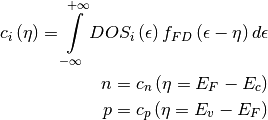
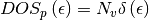
$n \left( E_F \right) = \int_{-\infty}^{+\infty} DOS_n \left( E - E_c \right) f_{FD}(E - E_F) dE$

In the valence band, almost all states are occupied by the electrons. It is therefore useful to track unoccupied states, holes, instead of the occupied states. The concentration of holes is given by:

$p \left( E_F \right) = \int_{-\infty}^{+\infty} DOS_p \left( E_v - E \right) \left[ 1 - f_{FD}(E - E_F) \right] dE$

Noting that

$1 - f_{FD}(E - E_F) = f_{FD}(E_F - E)$

and changing the integration variable, both concentrations can be written in a common form as:

(1)¶ $c_i \left( \eta \right) = \int\limits_{-\infty}^{+\infty} DOS_i \left(\epsilon \right) f_{FD} \left( \epsilon - \eta \right) d \epsilon n = c_n \left( \eta = E_F - E_c \right) p = c_p \left( \eta = E_v - E_F \right)$

Practical note: The SI base unit of energy is Joule (J), however the energies such as $E_F$ are very small and should be expressed in electronvolts (eV). The SI basic unit of concentration is $\mathrm{meter^{-3}}$ , although $\mathrm{{cm}^{-3}}$ is often encountered. The value of $k_B T$ at the room temperature is approximately 26 meV. The SI unit of temperature is Kelvin, $27^{\circ} \mathrm{C} \approx 300 \mathrm{K}$ .

Band energies¶

In an idealized case, the energies $E_c$ and $E_v$ of the conduction and valence bands are

(2)¶ $E_c = -q \psi - \chi E_v = E_c - E_g$

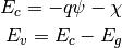
where $\chi > 0$ is the electron affinity energy, and $E_g > 0$ is the bandgap energy. $\psi$ is the electrostatic potential. q is the elementary charge.

Electrostatic potential¶

The electric field $\mathbf{E}$ is related to the elestrostatic potential $\psi$ as

(3)¶ $\mathbf{E} = - \nabla \psi$

In linear, isotropic, homogeneous medium the electric displacement field is

$\mathbf{D} = \varepsilon \mathbf{E}$

with permittivity

$\varepsilon = \varepsilon_0 \varepsilon_r$

where $\varepsilon_0$ is the vacuum permittivity, and $\varepsilon_r$ is the relative permittivity of the material.

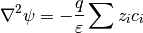
The electric displacement field satisfies the electric the Gauss’s equation

(4)¶ $\nabla \cdot \mathbf{D} = \rho_f$

where $\rho_f$ is the density of free charge

$\rho_f = q \left( p - n + \dots \right)$

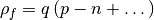
with $q$ denoting the elementary charge. Above, $\dots$ denotes other charges, such as ionized dopants.

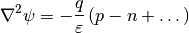
Combining the above equations gives the usual Poisson’s equation for electrostatics:

(5)¶ $\nabla^2 \psi = - \frac{q}{\varepsilon} \left( p - n + \dots \right)$

The SI unit of electrostatic potential is Volt, and the unit of electric field is Volt/meter. The unit of permittivity is Farad/meter. The unit of charge density is $\mathrm{Coulomb/{{meter}^3}}$ .

Approximation for low concentrations¶

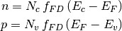
If the concentration of charge carriers is low enough, only states on the edge of band gap are important. In such case, the density of states can be assumed as a sharp energetic level,

$DOS_n \left( \epsilon \right) = N_c \delta \left( \epsilon \right)$

in case of electrons and

$DOS_p \left( \epsilon \right) = N_v \delta \left( \epsilon \right)$

in case of holes. Substiting into (1) gives

$n = N_c\, f_{FD} \left( E_c - E_F \right) p = N_v\, f_{FD} \left( E_F - E_v \right)$

At low charge carrier concentrations, Fermi-Dirac distribution $f_{FD}$ is simplified as

$f_{FD}(x)=\frac{1}{1+\exp \frac{x}{k_B T}} \approx \exp -\frac{x}{k_B T}$

The approximation is considered valid when $x > 4 k_B T$ .

Approximate charge carrier concentrations are

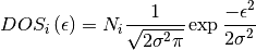
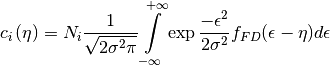
(6)¶ $n = N_c \exp \frac{E_F - E_c}{k_B T} p = N_v \exp \frac{E_v - E_F}{k_B T}$

Gaussian density of states¶

In the case of Gaussian DOS, the density of states shape function $DOS_i$ is the Gaussian distribution function scaled by total density of states $N_i$ :

$DOS_i \left( \epsilon \right) = N_i \frac{1}{\sqrt{2 \sigma^2 \pi}} \exp \frac{-\epsilon^2}{2 \sigma^2}$

Concentrations of species are given by integral

$c_i \left( \eta \right) = N_i \frac{1}{\sqrt{2 \sigma^2 \pi}} \int\limits_{-\infty}^{+\infty} \exp \frac{-\epsilon^2}{2 \sigma^2} f_{FD}(\epsilon - \eta) d \epsilon$

Conservation equation¶

The conservation equation is:

$\frac{\partial c_i}{\partial t} + \nabla \cdot \mathbf{j_i} = S_i$

where $c_i$ denotes the concentration, $t$ is time, and $j_i$ is the flux density. $S_i$ denotes source term, which is positive for generating particles, and negative for sinking particles of type i. The SI unit of source term is $\mathrm{1/\left({meter}^3 second\right)}$ .

The conservation equation must be satisfied for each species separately. In the case of transport of electrons and holes, this gives

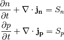
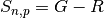
(7)¶ $\frac{\partial n}{\partial t} + \nabla \cdot \mathbf{j_n} = S_n \frac{\partial p}{\partial t} + \nabla \cdot \mathbf{j_p} = S_p$

where the source S term contains for example generation $G$ and recombination $R$ terms

$S_{n,p} = G - R$

The conservation of electric charge must be satisfied everywhere. Therefore, the source terms acting at given point must not create a net electric charge. In the case of system of electron and holes, this requires

$S_n = S_p$

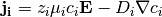
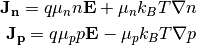
Current density¶

Current density $\mathbf{J_i}$ is related to the density flux $\mathbf{j_i}$ by the charge of single particle $z_i q$ . Obviously, for electrons $z = -1$ and for holes $z=1$ , therefore

(8)¶ $\mathbf{J_n} = -q \mathbf{j_n} \mathbf{J_p} = q \mathbf{j_p}$

Note that a convention is adopted to denote the electric current with uppercase letter $\mathbf{J}$ , and the flux density with lowercase letter $\mathbf{j}$ . The SI unit of density flux $\mathbf{j_i}$ is $\mathrm{1/({meter}^2\, second)}$ , while the unit of electric current density $\mathbf{J_i}$ is $\mathrm{Amper / {meter}^2}$ .

Equilibrium conditions¶

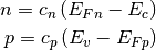
In the equilibrium conditions, Fermi level energy $E_F$ has the same value everywhere. The electrostatic potential $\psi$ can vary, and the density of free charge $\rho_f$ does not need to be zero. Equations (1), (2), (4) are satisfied simultaneously. The current flux, the source terms, and the time dependence are all zeros, so conservation (7) is trivially satisfied.

Nonequilibrium conditions¶

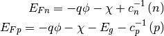
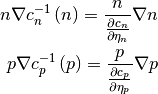
In the non-equilibrium conditions, the transport is introduced as a perturbation from equilibrium. The Fermi energy level is replaced with quasi Fermi level, which is different for each species. In (1), the equilibrium Fermi level for electrons $E_F$ is replaced with a quasi Fermi level $E_{Fn}$ . Similarly,, the equilibrium Fermi level for holes is replaced wuth quasi Fermi level for holes $E_{Fp}$ , giving

(9)¶ $n = c_n \left( E_{Fn} - E_c \right) p = c_p \left( E_v - E_{Fp} \right)$

Quasi Fermi levels have associated quasi Fermi potential according to the formula for energy of an electron in electrostatic field $E_F=-q \phi$ :

(10)¶ $E_{Fn} = -q \phi_n E_{Fp} = -q \phi_v$

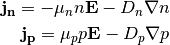
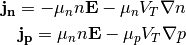
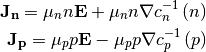
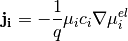
The transport is modeled by approximating electric current density as

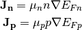
(11)¶ $\mathbf{J_n} = \mu_n n \nabla E_{Fn} \mathbf{J_p} = \mu_p p \nabla E_{Fp}$

where $\mu$ denotes the respective mobilities. The SI unit of mobility is $\mathrm{{meter}^2/(Volt\, second)}$ , although $\mathrm{cm^2/(V\, s)}$ is often used.

Equations (2), (5), (9), (11), (7) are simultaneously satisfied in non-equilibrium conditions.

Drift-diffusion system¶

Standard form of density fluxes in the drift-diffusion system is

(12)¶ $\mathbf{j_n} = - \mu_n n \mathbf{E} - D_n \nabla n \mathbf{j_p} = \mu_p p \mathbf{E} - D_p \nabla p$

or more generally, allowing arbitrary charge $z_i q$ per particle

(13)¶ $\mathbf{j_i} = z_i \mu_i c_i \mathbf{E} - D_i \nabla c_i$

$D_i$ is the diffusion coefficient, with SI unit $\mathrm{{meter}^2 {second}^{-1}}$ .

Drift-diffusion system: low concentration limit¶

To obtain the conventional drift-diffusion formulation (12), the the low concentration approximation (6) should be used. After introducing quasi Fermi levels, as it is done in (9), one obtains

$n = N_c \exp \frac{E_{Fn} - E_c}{k_B T} p = N_v \exp \frac{E_v - E_{Fp}}{k_B T}$

From that, the quasi Fermi energies are calculated as

$E_{Fn} = E_c + k_B T \log \frac{n}{N_c} E_{Fp} = E_v - k_B T \log \frac{p}{N_v}$

Using (2), and assuming constant ionization potential $\nabla \chi = 0$ , bandgap $\nabla E_g = 0$ , constant total densities of states $\nabla N_c = \nabla N_V = 0$ , and constant temperature $\nabla T = 0$ , substituting into (11), and using (3)

$\mathbf{J_n} = q \mu_n n \mathbf{E} + \mu_n k_B T \nabla n \mathbf{J_p} = q \mu_p p \mathbf{E} - \mu_p k_B T \nabla p$

In terms of density flux (8), this reads

(14)¶ $\mathbf{j_n} = - \mu_n n \mathbf{E} - \mu_n V_T \nabla n \mathbf{j_p} = \mu_n n \mathbf{E} - \mu_p V_T \nabla p$

where thermal voltage

$V_T = \frac{k_B T}{q}$

Einstein’s relation¶

Equation (14) is written in the standard drift-diffusion form (12) when the diffusion coefficient satisfies

(15)¶ $\frac{D_{n,p}}{\mu_{n,p}} = V_T$

This is called Einstein’s relation.

Drift-diffusion system: general case¶

Using functions defined in (1), bands (2) and approximation (9)

$E_{Fn} = -q \phi - \chi + c_n^{-1} \left( n \right) E_{Fp} = -q \phi - \chi - E_g - c_p^{-1} \left( p \right)$

current densities under assumptions 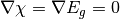$\nabla \chi = \nabla E_g = 0$ are

(16)¶ $\mathbf{J_n} = \mu_n n \mathbf{E} + \mu_n n \nabla c_n^{-1} \left( n \right) \mathbf{J_p} = \mu_p p \mathbf{E} - \mu_p p \nabla c_p^{-1} \left( p \right)$

Generalized Einstein’s relation¶

In equation (16), assuming $\nabla T = \nabla N_c = \nabla N_v = 0$

$n \nabla c_n^{-1} \left( n \right) = \frac{n}{\frac{\partial c_n}{\partial \eta_n}} \nabla n p \nabla c_p^{-1} \left( p \right) = \frac{p}{\frac{\partial c_p}{\partial \eta_p}} \nabla p$

In order to express equation (16) in the standard drift-diffusion form (12), the diffusion coefficient must satisfy

$\frac{D_i}{\mu_i} = \frac{1}{q} \frac{c_i}{\frac{\partial c_i}{\partial{\eta_i}}}$

This is so called generalized Einstein’s relation .

Intrinsic concentrations¶

Intrinsic concentrations $n_i$ , $p_i$ , and intrinsic Fermi level $E_{Fi}$ satisfy electric neutrality conditions

$n_i = c_n \left( E_{Fi} - E_c \right ) p_i = c_p \left( E_v - E_{Fi} \right) n_i = p_i$

Direct recombination¶

Direct recombination introduces source term

$R = \beta \left( n p - n_i p_i \right)$

where $\beta$ can be chosen freely.

Unidimensional form¶

By substituting $\nabla \rightarrow \frac{\partial}{\partial x}$ and $\nabla^2 \rightarrow \frac{\partial^2}{\partial x^2}$ , the equations (5), (7), (12) of the basic drift-diffusion device model are

$\frac{\partial^2 \psi}{\partial x^2} = - \frac{q}{\varepsilon} \left( p - n + \dots \right) E = - \frac{\partial{\psi}}{\partial{x}} j_n = - \mu_n n E - D_n \nabla \frac{\partial{n}}{\partial{x}} j_p = \mu_p p E - D_p \nabla \frac{\partial{p}}{\partial{x}} \frac{\partial n}{\partial t} + \frac{\partial{j_n}}{\partial{x}} = G - R \frac{\partial p}{\partial t} + \frac{\partial{j_p}}{\partial{x}} = G - R$

Total electric current density¶

Total electric current $\mathbf{J}$ is a sum of currents due to transport of each species and the displacement current $\mathbf{J_d}$

$\mathbf{J} = \mathbf{J_n} + \mathbf{J_p} + \mathbf{J_d} + \dots \mathbf{J_d} = \frac{\partial \mathbf{D}}{\partial t}$

Total electric current satisfies the conservation law

$\nabla \cdot \mathbf{J} = 0$

This can be verified by taking time derivative (4), using (7) and considering that the sum of all charge created by the source terms must be zero.

Electrode current¶

Current $I_\alpha$ passing through a surface $\Gamma_\alpha$ of electrode $\alpha$ is

(17)¶ $I_{\alpha}=\int_{\Gamma_\alpha}\boldsymbol{J}\cdot d\mathbf{S}$

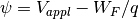
Metal¶

In metal, the relation between the electrostatic potential $\psi$ , the workfunction energy $W_F > 0$ and the Fermi level $E_F$ is

$E_F = -q \psi - W_F$

On the other hand, the Fermi potential corresponds to the applied voltage $V_{appl}$

$E_F = -q V_{appl}$

This leads to electrostatic potential at metal surface

$\psi = V_{appl} - W_F / q$

Ohmic contact¶

Ohmic contact is an idealization assuming that there is no charge accumulation at the contact, and the applied voltage $V_{appl}$ is equal to quasi Fermi potentials (10) of charged species

$\phi_n = V_{appl} \phi_p = V_{appl} n + N_A^{-} = p + N_D^{+}$

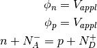
Above three conditions uniquely determine the charge concentrations $n$ , $p$ , and the electrostatic potential $\psi$ at the contact.

Electrochemical transport¶

Electrochemical potential for ionic species is

$\mu_i^{el} = z_i q \psi + k_B T \log c_i + \dots$

It should be noticed that so defined “potential” has the unit of energy, unlike the electrostatic potential and quasi Fermi potentials. Above $\dots$ denote corrections, for example due to steric interactions. Electrochemical potential $\mu_i^{el}$ should not be confused with mobility $\mu_i$ .

Density flux is approximated as

$\mathbf{j_i} = - \frac{1}{q} \mu_i c_i \nabla \mu_i^{el}$

yielding the standard form (13) using Einstein’s relation (15).

Electrochemical species should be included in Poisson’s equation, by including proper source terms of form $q z_i c_i$ . A variant of Poisson’s equation (5) where are free charges are ions can be written as

$\nabla^2 \psi = - \frac{q}{\varepsilon} \sum z_i c_i$

Steric corrections¶

To account for finite size of ions, the electrochemical potential in the form introduced in [LE13] is useful

$\mu_i^{el} = z_i q \psi + k_B T \log \frac{v_i c_i}{\Gamma}$

where $v_i$ denotes volume of particle of type $i$ . $\Gamma$ is the unoccupied fraction of space

$\Gamma = 1 - \sum_k v_k c_k$

where summing is taken over all species occupying space, including solvent.

[LE13]

Jinn-Liang Liu and Bob Eisenberg. Correlated Ions in a Calcium Channel Model: A Poisson–Fermi Theory. The Journal of Physical Chemistry B, 117(40):12051–12058, 2013. PMID: 24024558. URL: https://doi.org/10.1021/jp408330f, arXiv:https://doi.org/10.1021/jp408330f, doi:10.1021/jp408330f.